global TOMAWAC simulations

We'll generate a world contiguous mesh for global wave simulations.

install base environment

To be able to run this notebook, first install the pre-requisites for seamsh:

mamba create -n tomawac_mesh gdal gmsh scipy python=3.12

Optionally

create then a virtual environment on top of conda:

python -mvenv .venv 
source .venv/bin/activate

install libraries

pip install -e .

You're ready to run the notebook, and generate different version of the mesh.

This notebook contains to following sections:

  1. gather data:
    • A. GEBCO bathy through seareport_data
    • B. coastlines from natural earth coasltines
  2. Prepare the distance fields from the above data
    • only coastline is used to constrain with the Distance from the shore, but you can activate more contraints if necessary
  3. Mesh
  4. Interpolate bathy onto the mesh
  5. Convert to Selafin (using xarray-selafin available via pip)
  6. Generate the CLI file
  7. Interpolate ERA5 wind data onto the mesh
  8. Convert to wind Selafin binary
  9. Visualise TOMAWAC results directly in the notebook: WAC_global

1 - Generate the mesh

Particularities of the meshes available in the mesh/ folder:

  1. For TOMAWAC simulations, I needed to add a hole in the pole. Only because of the triangle(s) that contain the pole (bug in routine GEOELT.f).
  2. The mesh is contiguous, e.g. it wrap around the globe and the triangles at the dateline (+/- 180°) are connected alltogether.
  3. The only constraint for the mesh size is the distance from the coast. You can activate the wavelength contrainst (proportional to sqrt(depth)) or the bathy gradient constraint.

2 - Run the model

You will need to compile and run TELEMAC from the main branch, because it contains the latest version of 1D time series exports, very useful for global model analysis (and comparison against buoys).

All the modified routines to run TOMAWAC global are in wac/princi/ folder.

Look for SEB or TOM for the modified parts of the source code.

Get the whole project:

available on Google drive : https://drive.google.com/drive/folders/1SMNkHymAeuRfKh27pwPf7TgdIlOhTBvI?usp=sharing

In [1]:
import seamsh
import numpy as np
import xarray as xr
import seareport_data as D
import utils
import hvplot.pandas
import hvplot.xarray

Mesh settings

here are the main parameters used for the mesher settings:

In [2]:
# Meshing parameters for contributions
OPTS = {
    "max": 150000,      # max resolution
    "min": 10000,        # min resolution
    "dist": 0.15,       # The rate of expansion in decimal percent from the shoreline
    "wl": 50,           # (not used here) number of element to resolve WL
    "m2": 12.42 * 3600, # (not used here) for wavelength: M2 period in seconds
    "g": 9.81,          # (not used here) for wavelength: m/s^2
    "slope": 5,         # (not used here) number of element to resolve bathy gradient
    "grade": 1.5,       # the rate of growth in decimal percent
}
REMOVE_POLE = True      # for tomawac simulations

Coastlines

In [3]:
SHP_IN = "ne_10m_coastline/ne_10m_coastline.shp"
SHPOUT = "ne_10m_coastline/ne_10m_coastline_poly.shp"
POLE= "ne_10m_coastline/pole_ring.shp"
utils.get_ne_coastline(SHP_IN)
utils.remove_small_islands(SHP_IN, SHPOUT, OPTS['min'])
utils.add_hole_in_pole(POLE)

define the CRS for the meshing

In [ ]:
from osgeo import osr
domain_srs = osr.SpatialReference()
domain_srs.ImportFromProj4("+ellps=WGS84 +proj=stere +lat_0=90")
# "Cartesian" projection (i.e. no projection) is used to compute the distance to the coast.
cart_srs = osr.SpatialReference()
cart_srs.ImportFromProj4("+ellps=WGS84 +proj=cart +units=m +x_0=0 +y_0=0")
wgs84_srs = osr.SpatialReference()
wgs84_srs.ImportFromProj4("+ellps=WGS84 +proj=longlat +datum=WGS84 +no_defs")

Distance field

In [ ]:
domain = seamsh.geometry.Domain(domain_srs)
domain.add_boundary_curves_shp(SHPOUT, "featurecla", seamsh.geometry.CurveType.POLYLINE)
dist_coast = seamsh.field.Distance(domain, OPTS["min"]/2, projection=cart_srs)

Bathy field (not used here)

In [6]:
bathy = D.gebco_ds("sub_ice")
bathy_subset = bathy.isel(lon=slice(0,-1,10), lat=slice(0,-1,10))
bathy_grad = utils.calc_gradient(bathy_subset, 'elevation')
bathy_grad
Out[6]:
<xarray.Dataset> Size: 373MB
Dimensions:    (lat: 4320, lon: 8640)
Coordinates:
  * lon        (lon) float64 69kB -180.0 -180.0 -179.9 ... 179.9 179.9 180.0
  * lat        (lat) float64 35kB -90.0 -89.96 -89.91 ... 89.88 89.92 89.96
Data variables:
    crs        |S1 1B ...
    elevation  (lat, lon) int16 75MB -18 -18 -18 -18 ... -4212 -4212 -4212 -4212
    gradient   (lat, lon) float64 299MB 0.02388 0.02409 ... 2.912e-08 2.912e-08
Attributes: (12/36)
    title:                           The GEBCO_2025 Grid - a continuous terra...
    summary:                         The GEBCO_2025 Grid is a continuous, glo...
    keywords:                        BATHYMETRY/SEAFLOOR TOPOGRAPHY, DIGITAL ...
    Conventions:                     CF-1.6, ACDD-1.3
    id:                              DOI: 10.5285/37c52e96-24ea-67ce-e063-708...
    naming_authority:                https://dx.doi.org
    ...                              ...
    geospatial_vertical_units:       meters
    geospatial_vertical_resolution:  1.0
    geospatial_vertical_positive:    up
    identifier_product_doi:          DOI: 10.5285/37c52e96-24ea-67ce-e063-708...
    references:                      DOI: 10.5285/37c52e96-24ea-67ce-e063-708...
    node_offset:                     1.0
xarray.Dataset
    • lat: 4320
    • lon: 8640
    • lon
      (lon)
      float64
      -180.0 -180.0 ... 179.9 180.0
      standard_name :
      longitude
      long_name :
      longitude
      units :
      degrees_east
      axis :
      X
      sdn_parameter_urn :
      SDN:P01::ALONZZ01
      sdn_parameter_name :
      Longitude east
      sdn_uom_urn :
      SDN:P06::DEGE
      sdn_uom_name :
      Degrees east
      array([-179.997917, -179.95625 , -179.914583, ...,  179.877083,  179.91875 ,
              179.960417], shape=(8640,))
    • lat
      (lat)
      float64
      -90.0 -89.96 -89.91 ... 89.92 89.96
      standard_name :
      latitude
      long_name :
      latitude
      units :
      degrees_north
      axis :
      Y
      sdn_parameter_urn :
      SDN:P01::ALATZZ01
      sdn_parameter_name :
      Latitude north
      sdn_uom_urn :
      SDN:P06::DEGN
      sdn_uom_name :
      Degrees north
      array([-89.997917, -89.95625 , -89.914583, ...,  89.877083,  89.91875 ,
              89.960417], shape=(4320,))
    • crs
      ()
      |S1
      ...
      grid_mapping_name :
      latitude_longitude
      epsg_code :
      EPSG:4326
      inverse_flattening :
      298.257223563
      semi_major_axis :
      6378137.0
      [1 values with dtype=|S1]
    • elevation
      (lat, lon)
      int16
      -18 -18 -18 ... -4212 -4212 -4212
      standard_name :
      height_above_mean_sea_level
      long_name :
      Elevation relative to sea level
      units :
      m
      grid_mapping :
      crs
      sdn_parameter_urn :
      SDN:P01::BATHHGHT
      sdn_parameter_name :
      Sea floor height (above mean sea level) {bathymetric height}
      sdn_uom_urn :
      SDN:P06::ULAA
      sdn_uom_name :
      Metres
      array([[  -18,   -18,   -18, ...,   -18,   -18,   -18],
             [   92,    93,    93, ...,    92,    92,    92],
             [   64,    64,    64, ...,    64,    64,    64],
             ...,
             [-4214, -4214, -4214, ..., -4215, -4215, -4214],
             [-4221, -4221, -4221, ..., -4220, -4221, -4221],
             [-4212, -4212, -4212, ..., -4212, -4212, -4212]],
            shape=(4320, 8640), dtype=int16)
    • gradient
      (lat, lon)
      float64
      0.02388 0.02409 ... 2.912e-08
      array([[2.38753548e-02, 2.40924035e-02, 2.40924035e-02, ...,
              2.38753548e-02, 2.38753548e-02, 2.38753548e-02],
             [8.90164244e-03, 8.89965761e-03, 8.89899590e-03, ...,
              8.89899590e-03, 8.89899590e-03, 8.89899590e-03],
             [1.03098123e-02, 1.05268610e-02, 1.05268610e-02, ...,
              1.03098123e-02, 1.03098123e-02, 1.03098123e-02],
             ...,
             [1.02977194e-06, 8.82661661e-07, 8.82661661e-07, ...,
              1.17688221e-06, 1.04022674e-06, 1.07097899e-06],
             [5.69654472e-08, 5.69654472e-08, 5.69654472e-08, ...,
              9.00702810e-08, 9.00702810e-08, 5.69654472e-08],
             [2.91211921e-08, 2.91211921e-08, 2.91211921e-08, ...,
              2.58855041e-08, 2.91211921e-08, 2.91211921e-08]],
            shape=(4320, 8640))
    • lon
      PandasIndex
      PandasIndex(Index([-179.99791666666667,          -179.95625, -179.91458333333333,
             -179.87291666666667,          -179.83125, -179.78958333333333,
             -179.74791666666667,          -179.70625, -179.66458333333333,
             -179.62291666666667,
             ...
              179.58541666666667,   179.6270833333333,           179.66875,
              179.71041666666667,   179.7520833333333,           179.79375,
              179.83541666666667,   179.8770833333333,           179.91875,
              179.96041666666667],
            dtype='float64', name='lon', length=8640))
    • lat
      PandasIndex
      PandasIndex(Index([-89.99791666666667,          -89.95625, -89.91458333333334,
             -89.87291666666667,          -89.83125, -89.78958333333334,
             -89.74791666666667,          -89.70625, -89.66458333333334,
             -89.62291666666667,
             ...
              89.58541666666667,  89.62708333333333,  89.66874999999999,
              89.71041666666667,  89.75208333333333,  89.79374999999999,
              89.83541666666667,  89.87708333333333,  89.91874999999999,
              89.96041666666667],
            dtype='float64', name='lat', length=4320))
  • title :
    The GEBCO_2025 Grid - a continuous terrain model for oceans and land at 15 arc-second intervals
    summary :
    The GEBCO_2025 Grid is a continuous, global terrain model for ocean and land with a spatial resolution of 15 arc seconds.The grid uses as a base-map Version 2.7 of the SRTM15+ data set (Tozer et al, 2019). This data set is a fusion of land topography with measured and estimated seafloor topography. It is augmented with gridded bathymetric data sets developed as part of the Nippon Foundation-GEBCO Seabed 2030 Project.
    keywords :
    BATHYMETRY/SEAFLOOR TOPOGRAPHY, DIGITAL ELEVATION/DIGITAL TERRAIN MODELS
    Conventions :
    CF-1.6, ACDD-1.3
    id :
    DOI: 10.5285/37c52e96-24ea-67ce-e063-7086abc05f29
    naming_authority :
    https://dx.doi.org
    history :
    Information on the development of the data set and the source data sets included in the grid can be found in the data set documentation available from https://www.gebco.net
    source :
    The GEBCO_2025 Grid is the 2025 release of the global bathymetric product published by the General Bathymetric Chart of the Oceans (GEBCO) and has been developed through the Nippon Foundation-GEBCO Seabed 2030 Project. This is a collaborative project between the Nippon Foundation of Japan and GEBCO. The Seabed 2030 Project aims to bring together all available bathymetric data to produce the definitive map of the world ocean floor and make it available to all.
    comment :
    The data in the GEBCO_2025 Grid should not be used for navigation or any purpose relating to safety at sea.
    license :
    The GEBCO Grid is placed in the public domain and may be used free of charge. Use of the GEBCO Grid indicates that the user accepts the conditions of use and disclaimer information: https://www.gebco.net/
    date_created :
    2025-07-18
    creator_name :
    GEBCO through the Nippon Foundation-GEBCO Seabed 2030 Project
    creator_email :
    gdacc@seabed2030.org
    creator_url :
    https://www.gebco.net
    institution :
    On behalf of the General Bathymetric Chart of the Oceans (GEBCO), the data are held at the British Oceanographic Data Centre (BODC).
    project :
    Nippon Foundation - GEBCO Seabed2030 Project
    creator_type :
    International organisation
    geospatial_bounds :
    [-180. -90. 180. 90.]
    geospatial_bounds_crs :
    WGS84
    geospatial_bounds_vertical_crs :
    EPSG:5831
    geospatial_lat_min :
    -90.0
    geospatial_lat_max :
    90.0
    geospatial_lat_units :
    degrees_north
    geospatial_lat_resolution :
    0.004166666666666667
    geospatial_lon_min :
    -180.0
    geospatial_lon_max :
    180.0
    geospatial_lon_units :
    degrees_east
    geospatial_lon_resolution :
    0.004166666666666667
    geospatial_vertical_min :
    -10930.0
    geospatial_vertical_max :
    8627.0
    geospatial_vertical_units :
    meters
    geospatial_vertical_resolution :
    1.0
    geospatial_vertical_positive :
    up
    identifier_product_doi :
    DOI: 10.5285/37c52e96-24ea-67ce-e063-7086abc05f29
    references :
    DOI: 10.5285/37c52e96-24ea-67ce-e063-7086abc05f29
    node_offset :
    1.0
In [ ]:
! mkdir -p data
In [ ]:
BATHY = "data/gebco_2024_1000_4k.tif"
BATHY_GRADIENT = "data/gebco_2024_grad_smooth_1000_4k.tif"
utils.to_raster(bathy_subset.elevation, BATHY)
utils.to_raster(bathy_grad.gradient, BATHY_GRADIENT)
In [ ]:
bath_field = seamsh.field.Raster(BATHY)
bath_field._projection = osr.SpatialReference()
bath_field._projection.ImportFromProj4("+proj=longlat +ellps=WGS84 +datum=WGS84 +no_defs")
grad_field = seamsh.field.Raster(BATHY_GRADIENT)
grad_field._projection = osr.SpatialReference()
grad_field._projection.ImportFromProj4("+proj=longlat +ellps=WGS84 +datum=WGS84 +no_defs")
# %%

MESH

Mesh size function

In [10]:
# it is necessary to convert the mesh size to stereographic coordinates
def mesh_size(x, projection,R = 6371000):
    depth = bath_field(x, projection)
    depth[depth>0] = 0
    grad = grad_field(x, projection)
    lon, lat = utils.stereo_to_wgs84(x, source_epsg=projection)
    s_wl = OPTS["m2"] / OPTS["wl"] * np.sqrt(9.81 * - depth)
    s_wl = np.clip(s_wl, OPTS["min"]*2,None)
    s_grad = abs(depth) / (grad + 1e-10)*(2*np.pi / OPTS["slope"])
    s_grad = np.clip(s_grad, OPTS["min"]*3,None)
    s_coast = dist_coast(x, projection)* OPTS["grade"] + OPTS["min"]

    # s_final = np.c_[s_coast, s_wl, s_grad].min(axis=1)
    s_final = s_coast

    stereo_factor = 2/(1+x[:,0]**2/R**2+x[:,1]**2/R**2) * (3/4*np.cos(np.deg2rad(lat+90))+5/4)
    return np.clip(s_final,OPTS["min"],OPTS["max"])/stereo_factor

Coarsen boundaries

In [ ]:
coarse = seamsh.geometry.coarsen_boundaries(domain, (0, 0), domain_srs, mesh_size)
if REMOVE_POLE:
    coarse.add_boundary_curves_shp(POLE,"featurecla", seamsh.geometry.CurveType.POLYLINE)
else: 
    x = [[0., 0.]]
    coarse.add_interior_points(x,"featurecla",domain_srs)

finally mesh

In [12]:
seamsh.gmsh.mesh(
    coarse, 
    "natural_earth.msh", 
    mesh_size, 
    output_srs=domain_srs,
    intermediate_file_name="-",
    # binary=True
)
seamsh.gmsh.reproject("natural_earth.msh", domain_srs, "natural_earth_wgs84.msh", wgs84_srs)
 * Generate mesh * 
Build topology
Build gmsh model
Build mesh size field
Mesh with gmsh
Write "natural_earth.msh" (msh version 4.1)

Interpolate Bathy

In [13]:
import gmsh
gmsh.open("natural_earth_wgs84.msh")
tri_i, tri_n = gmsh.model.mesh.getElementsByType(2)
tri_n = tri_n.reshape([-1, 3])
node_i, nodes, _ = gmsh.model.mesh.getNodes()
nodes = nodes.reshape([-1, 3])
x = nodes[:, 0]
y = nodes[:, 1]
z = nodes[:, 2]
element = np.subtract(tri_n, 1)
In [14]:
subset = bathy.isel(lon=slice(0, -1, 10), lat=slice(0, -1, 10)).pad(lon=(1,1),lat=(1,1),mode="edge")
lon_values = subset.lon.values
lat_values = subset.lat.values
lon_values[-1] = 180.0
lon_values[0] = -180.0
lat_values[-1] = 90.0
lat_values[0] = -90.0
subset = subset.assign_coords(lon=lon_values,lat=lat_values)
subset
Out[14]:
<xarray.Dataset> Size: 75MB
Dimensions:    (lat: 4322, lon: 8642)
Coordinates:
  * lon        (lon) float64 69kB -180.0 -180.0 -180.0 ... 179.9 180.0 180.0
  * lat        (lat) float64 35kB -90.0 -90.0 -89.96 -89.91 ... 89.92 89.96 90.0
Data variables:
    crs        |S1 1B ...
    elevation  (lat, lon) int16 75MB -18 -18 -18 -18 ... -4212 -4212 -4212 -4212
Attributes: (12/36)
    title:                           The GEBCO_2025 Grid - a continuous terra...
    summary:                         The GEBCO_2025 Grid is a continuous, glo...
    keywords:                        BATHYMETRY/SEAFLOOR TOPOGRAPHY, DIGITAL ...
    Conventions:                     CF-1.6, ACDD-1.3
    id:                              DOI: 10.5285/37c52e96-24ea-67ce-e063-708...
    naming_authority:                https://dx.doi.org
    ...                              ...
    geospatial_vertical_units:       meters
    geospatial_vertical_resolution:  1.0
    geospatial_vertical_positive:    up
    identifier_product_doi:          DOI: 10.5285/37c52e96-24ea-67ce-e063-708...
    references:                      DOI: 10.5285/37c52e96-24ea-67ce-e063-708...
    node_offset:                     1.0
xarray.Dataset
    • lat: 4322
    • lon: 8642
    • lon
      (lon)
      float64
      -180.0 -180.0 ... 180.0 180.0
      array([-180.      , -179.997917, -179.95625 , ...,  179.91875 ,  179.960417,
              180.      ], shape=(8642,))
    • lat
      (lat)
      float64
      -90.0 -90.0 -89.96 ... 89.96 90.0
      array([-90.      , -89.997917, -89.95625 , ...,  89.91875 ,  89.960417,
              90.      ], shape=(4322,))
    • crs
      ()
      |S1
      ...
      grid_mapping_name :
      latitude_longitude
      epsg_code :
      EPSG:4326
      inverse_flattening :
      298.257223563
      semi_major_axis :
      6378137.0
      [1 values with dtype=|S1]
    • elevation
      (lat, lon)
      int16
      -18 -18 -18 ... -4212 -4212 -4212
      standard_name :
      height_above_mean_sea_level
      long_name :
      Elevation relative to sea level
      units :
      m
      grid_mapping :
      crs
      sdn_parameter_urn :
      SDN:P01::BATHHGHT
      sdn_parameter_name :
      Sea floor height (above mean sea level) {bathymetric height}
      sdn_uom_urn :
      SDN:P06::ULAA
      sdn_uom_name :
      Metres
      array([[  -18,   -18,   -18, ...,   -18,   -18,   -18],
             [  -18,   -18,   -18, ...,   -18,   -18,   -18],
             [   92,    92,    93, ...,    92,    92,    92],
             ...,
             [-4221, -4221, -4221, ..., -4221, -4221, -4221],
             [-4212, -4212, -4212, ..., -4212, -4212, -4212],
             [-4212, -4212, -4212, ..., -4212, -4212, -4212]],
            shape=(4322, 8642), dtype=int16)
    • lon
      PandasIndex
      PandasIndex(Index([             -180.0, -179.99791666666667,          -179.95625,
             -179.91458333333333, -179.87291666666667,          -179.83125,
             -179.78958333333333, -179.74791666666667,          -179.70625,
             -179.66458333333333,
             ...
               179.6270833333333,           179.66875,  179.71041666666667,
               179.7520833333333,           179.79375,  179.83541666666667,
               179.8770833333333,           179.91875,  179.96041666666667,
                           180.0],
            dtype='float64', name='lon', length=8642))
    • lat
      PandasIndex
      PandasIndex(Index([             -90.0, -89.99791666666667,          -89.95625,
             -89.91458333333334, -89.87291666666667,          -89.83125,
             -89.78958333333334, -89.74791666666667,          -89.70625,
             -89.66458333333334,
             ...
              89.62708333333333,  89.66874999999999,  89.71041666666667,
              89.75208333333333,  89.79374999999999,  89.83541666666667,
              89.87708333333333,  89.91874999999999,  89.96041666666667,
                           90.0],
            dtype='float64', name='lat', length=4322))
  • title :
    The GEBCO_2025 Grid - a continuous terrain model for oceans and land at 15 arc-second intervals
    summary :
    The GEBCO_2025 Grid is a continuous, global terrain model for ocean and land with a spatial resolution of 15 arc seconds.The grid uses as a base-map Version 2.7 of the SRTM15+ data set (Tozer et al, 2019). This data set is a fusion of land topography with measured and estimated seafloor topography. It is augmented with gridded bathymetric data sets developed as part of the Nippon Foundation-GEBCO Seabed 2030 Project.
    keywords :
    BATHYMETRY/SEAFLOOR TOPOGRAPHY, DIGITAL ELEVATION/DIGITAL TERRAIN MODELS
    Conventions :
    CF-1.6, ACDD-1.3
    id :
    DOI: 10.5285/37c52e96-24ea-67ce-e063-7086abc05f29
    naming_authority :
    https://dx.doi.org
    history :
    Information on the development of the data set and the source data sets included in the grid can be found in the data set documentation available from https://www.gebco.net
    source :
    The GEBCO_2025 Grid is the 2025 release of the global bathymetric product published by the General Bathymetric Chart of the Oceans (GEBCO) and has been developed through the Nippon Foundation-GEBCO Seabed 2030 Project. This is a collaborative project between the Nippon Foundation of Japan and GEBCO. The Seabed 2030 Project aims to bring together all available bathymetric data to produce the definitive map of the world ocean floor and make it available to all.
    comment :
    The data in the GEBCO_2025 Grid should not be used for navigation or any purpose relating to safety at sea.
    license :
    The GEBCO Grid is placed in the public domain and may be used free of charge. Use of the GEBCO Grid indicates that the user accepts the conditions of use and disclaimer information: https://www.gebco.net/
    date_created :
    2025-07-18
    creator_name :
    GEBCO through the Nippon Foundation-GEBCO Seabed 2030 Project
    creator_email :
    gdacc@seabed2030.org
    creator_url :
    https://www.gebco.net
    institution :
    On behalf of the General Bathymetric Chart of the Oceans (GEBCO), the data are held at the British Oceanographic Data Centre (BODC).
    project :
    Nippon Foundation - GEBCO Seabed2030 Project
    creator_type :
    International organisation
    geospatial_bounds :
    [-180. -90. 180. 90.]
    geospatial_bounds_crs :
    WGS84
    geospatial_bounds_vertical_crs :
    EPSG:5831
    geospatial_lat_min :
    -90.0
    geospatial_lat_max :
    90.0
    geospatial_lat_units :
    degrees_north
    geospatial_lat_resolution :
    0.004166666666666667
    geospatial_lon_min :
    -180.0
    geospatial_lon_max :
    180.0
    geospatial_lon_units :
    degrees_east
    geospatial_lon_resolution :
    0.004166666666666667
    geospatial_vertical_min :
    -10930.0
    geospatial_vertical_max :
    8627.0
    geospatial_vertical_units :
    meters
    geospatial_vertical_resolution :
    1.0
    geospatial_vertical_positive :
    up
    identifier_product_doi :
    DOI: 10.5285/37c52e96-24ea-67ce-e063-7086abc05f29
    references :
    DOI: 10.5285/37c52e96-24ea-67ce-e063-7086abc05f29
    node_offset :
    1.0
In [15]:
from scipy.interpolate import RegularGridInterpolator as RGI
RG = RGI((subset.lon, subset.lat), subset.elevation.data.T, method="linear")

export to Selafin

In [16]:
!mkdir -p mesh
In [17]:
from xarray_selafin.xarray_backend import SelafinAccessor
import pandas as pd

slf_ds = xr.Dataset(
    coords={
        "time": [pd.Timestamp.now()],
        "x": ("node", x),
        "y": ("node", y),
    },
    data_vars={
        "B" : (("time", "node"), [RG((x,y))])
    }
)
slf_ds.attrs['ikle2'] = element + 1
filebase = f"mesh/global_{OPTS["min"]/1000}-{int(OPTS["max"]/1000)}km-smo{OPTS["grade"]-1}-{len(slf_ds.x)}nodes"
slf_ds.selafin.write(filebase+".slf")
# export CLI file
_=utils.export_cli(slf_ds, filebase+".cli")
No description has been provided for this image
In [18]:
slf_ds
Out[18]:
<xarray.Dataset> Size: 3MB
Dimensions:  (time: 1, node: 133059)
Coordinates:
  * time     (time) datetime64[ns] 8B 2025-09-26T18:09:23.790500
    x        (node) float64 1MB -26.24 -156.1 -66.72 ... -2.335 110.9 -60.49
    y        (node) float64 1MB -58.48 -85.13 -78.44 -80.3 ... 49.1 79.26 9.148
Dimensions without coordinates: node
Data variables:
    B        (time, node) float64 1MB -155.3 -871.3 -361.1 ... -1.926e+03 -5.747
Attributes:
    ikle2:    [[106330 113322  86664]\n [  1957 124004  18862]\n [ 64490 1239...
xarray.Dataset
    • time: 1
    • node: 133059
    • time
      (time)
      datetime64[ns]
      2025-09-26T18:09:23.790500
      array(['2025-09-26T18:09:23.790500000'], dtype='datetime64[ns]')
    • x
      (node)
      float64
      -26.24 -156.1 ... 110.9 -60.49
      array([ -26.2413695 , -156.08769924,  -66.71829193, ...,   -2.33539665,
              110.86329715,  -60.49098148], shape=(133059,))
    • y
      (node)
      float64
      -58.48 -85.13 ... 79.26 9.148
      array([-58.48456893, -85.13375997, -78.44140748, ...,  49.09997673,
              79.26263522,   9.14774935], shape=(133059,))
    • B
      (time, node)
      float64
      -155.3 -871.3 ... -1.926e+03 -5.747
      array([[ -155.31735793,  -871.31227204,  -361.10873977, ...,
                -36.36330246, -1925.6432897 ,    -5.74699555]],
            shape=(1, 133059))
    • time
      PandasIndex
      PandasIndex(DatetimeIndex(['2025-09-26 18:09:23.790500'], dtype='datetime64[ns]', name='time', freq=None))
  • ikle2 :
    [[106330 113322 86664] [ 1957 124004 18862] [ 64490 123918 73975] ... [ 44037 44047 44035] [ 54690 64110 47369] [117263 120215 74571]]
In [19]:
filebase
Out[19]:
'mesh/global_10.0-150km-smo0.5-133059nodes'
In [ ]:
slf_ds.B.hvplot.scatter(
    x="x",
    y="y",
    c='B',
    cmap="fire",
    s=1,
    clim=(-5000, 0),
    ).opts(
        width=800,
        height=500,
    )
Out[ ]:
BokehModel(combine_events=True, render_bundle={'docs_json': {'77a0288a-0fd2-480d-92b0-03ec038329b6': {'version…

Interpolate wind

In [21]:
atm_nc = xr.open_dataset("data/era5_202307_uvp.nc")
atm_nc
Out[21]:
<xarray.Dataset> Size: 19GB
Dimensions:    (time: 744, latitude: 721, longitude: 1440)
Coordinates:
  * longitude  (longitude) float32 6kB 0.0 0.25 0.5 0.75 ... 359.2 359.5 359.8
  * latitude   (latitude) float32 3kB 90.0 89.75 89.5 ... -89.5 -89.75 -90.0
  * time       (time) datetime64[ns] 6kB 2023-07-01 ... 2023-07-31T23:00:00
Data variables:
    msl        (time, latitude, longitude) float64 6GB ...
    u10        (time, latitude, longitude) float64 6GB ...
    v10        (time, latitude, longitude) float64 6GB ...
Attributes:
    Conventions:  CF-1.6
    history:      2024-04-04 09:42:07 GMT by grib_to_netcdf-2.25.1: /opt/ecmw...
xarray.Dataset
    • time: 744
    • latitude: 721
    • longitude: 1440
    • longitude
      (longitude)
      float32
      0.0 0.25 0.5 ... 359.2 359.5 359.8
      units :
      degrees_east
      long_name :
      longitude
      array([0.0000e+00, 2.5000e-01, 5.0000e-01, ..., 3.5925e+02, 3.5950e+02,
             3.5975e+02], shape=(1440,), dtype=float32)
    • latitude
      (latitude)
      float32
      90.0 89.75 89.5 ... -89.75 -90.0
      units :
      degrees_north
      long_name :
      latitude
      array([ 90.  ,  89.75,  89.5 , ..., -89.5 , -89.75, -90.  ],
            shape=(721,), dtype=float32)
    • time
      (time)
      datetime64[ns]
      2023-07-01 ... 2023-07-31T23:00:00
      long_name :
      time
      array(['2023-07-01T00:00:00.000000000', '2023-07-01T01:00:00.000000000',
             '2023-07-01T02:00:00.000000000', ..., '2023-07-31T21:00:00.000000000',
             '2023-07-31T22:00:00.000000000', '2023-07-31T23:00:00.000000000'],
            shape=(744,), dtype='datetime64[ns]')
    • msl
      (time, latitude, longitude)
      float64
      ...
      units :
      Pa
      long_name :
      Mean sea level pressure
      standard_name :
      air_pressure_at_mean_sea_level
      [772450560 values with dtype=float64]
    • u10
      (time, latitude, longitude)
      float64
      ...
      units :
      m s**-1
      long_name :
      10 metre U wind component
      [772450560 values with dtype=float64]
    • v10
      (time, latitude, longitude)
      float64
      ...
      units :
      m s**-1
      long_name :
      10 metre V wind component
      [772450560 values with dtype=float64]
    • longitude
      PandasIndex
      PandasIndex(Index([   0.0,   0.25,    0.5,   0.75,    1.0,   1.25,    1.5,   1.75,    2.0,
               2.25,
             ...
              357.5, 357.75,  358.0, 358.25,  358.5, 358.75,  359.0, 359.25,  359.5,
             359.75],
            dtype='float32', name='longitude', length=1440))
    • latitude
      PandasIndex
      PandasIndex(Index([  90.0,  89.75,   89.5,  89.25,   89.0,  88.75,   88.5,  88.25,   88.0,
              87.75,
             ...
             -87.75,  -88.0, -88.25,  -88.5, -88.75,  -89.0, -89.25,  -89.5, -89.75,
              -90.0],
            dtype='float32', name='latitude', length=721))
    • time
      PandasIndex
      PandasIndex(DatetimeIndex(['2023-07-01 00:00:00', '2023-07-01 01:00:00',
                     '2023-07-01 02:00:00', '2023-07-01 03:00:00',
                     '2023-07-01 04:00:00', '2023-07-01 05:00:00',
                     '2023-07-01 06:00:00', '2023-07-01 07:00:00',
                     '2023-07-01 08:00:00', '2023-07-01 09:00:00',
                     ...
                     '2023-07-31 14:00:00', '2023-07-31 15:00:00',
                     '2023-07-31 16:00:00', '2023-07-31 17:00:00',
                     '2023-07-31 18:00:00', '2023-07-31 19:00:00',
                     '2023-07-31 20:00:00', '2023-07-31 21:00:00',
                     '2023-07-31 22:00:00', '2023-07-31 23:00:00'],
                    dtype='datetime64[ns]', name='time', length=744, freq=None))
  • Conventions :
    CF-1.6
    history :
    2024-04-04 09:42:07 GMT by grib_to_netcdf-2.25.1: /opt/ecmwf/mars-client/bin/grib_to_netcdf.bin -S param -o /cache/data5/adaptor.mars.internal-1712223465.2069833-14833-10-170b5d44-2e0e-42df-826b-56c1dd5e4490.nc /cache/tmp/170b5d44-2e0e-42df-826b-56c1dd5e4490-adaptor.mars.internal-1712222898.1675792-14833-10-tmp.grib
In [22]:
lon_values = atm_nc.longitude.values
lat_values = atm_nc.latitude.values
lon_values[-1] = 360.0
atm_nc = atm_nc.assign_coords(lon=lon_values)
In [23]:
atm_data = dict()

for var in ["msl", "u10", "v10"]: 
    RG = RGI((atm_nc.longitude, atm_nc.latitude), atm_nc[var].data.T, method="linear")
    atm_data[var] = RG((slf_ds.x.data % 360, slf_ds.y.data))

slf_wind =xr.Dataset(coords = {
    "x": ("node", slf_ds.x.data),
    "y": ("node", slf_ds.y.data),
    "time": atm_nc.time.data
    },
    data_vars={
        "PATM": (("node", "time"), atm_data["msl"]),
        "WINDX": (("node", "time"), atm_data["u10"]),
        "WINDY": (("node", "time"), atm_data["v10"]),
    }
)
slf_wind.attrs["ikle2"] = slf_ds.ikle2
slf_wind.attrs["variables"] = {'PATM': ('PATM', 'PASCAL'), 'WINDX': ('WINDX', 'M/S'), 'WINDY': ('WINDY', 'M/S')}
In [24]:
slf_wind.selafin.write(filebase+"_wind.slf")
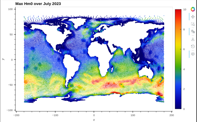
Inspect results

In [25]:
res2d = xr.open_dataset("wac/r2d_global_tom.slf")
res1d = xr.open_dataset("wac/r1d_global_tom.slf")
In [26]:
res2d.max(dim="time").WH.hvplot.scatter(x="x",
    y="y",
    c='WH',
    cmap="rainbow4",
    s=1,   
).opts(
    clim=(0, 10),
    width=800,
    height=500,
    title="Max Hm0 over July 2023"
)
Out[26]:
In [27]:
res1d.max(dim="time").WH.hvplot.scatter(x="x",
    y="y",
    c='WH',
    cmap="rainbow4",
    hover_cols=["node"]
).opts(
    clim=(0, 10),
    width=800,
    height=500,
    title="Max Hm0 over July 2023"
)
Out[27]:
In [28]:
res1d.isel(node=389).WH.hvplot(
).opts(
    width=800,
    height=500,
    title=f"Hm0 over July 2023, for station located at {res1d.isel(node=389).x.values:0.2f}°E, {res1d.isel(node=389).y.values:0.2f}°N"
)
Out[28]: